
Learning Objectives
Following this assignment students should be able to:
- start to combine multiple computing concepts to solve bigger problems
- start to debug errors in their code
- use good style
Reading
Lecture Notes
Exercises
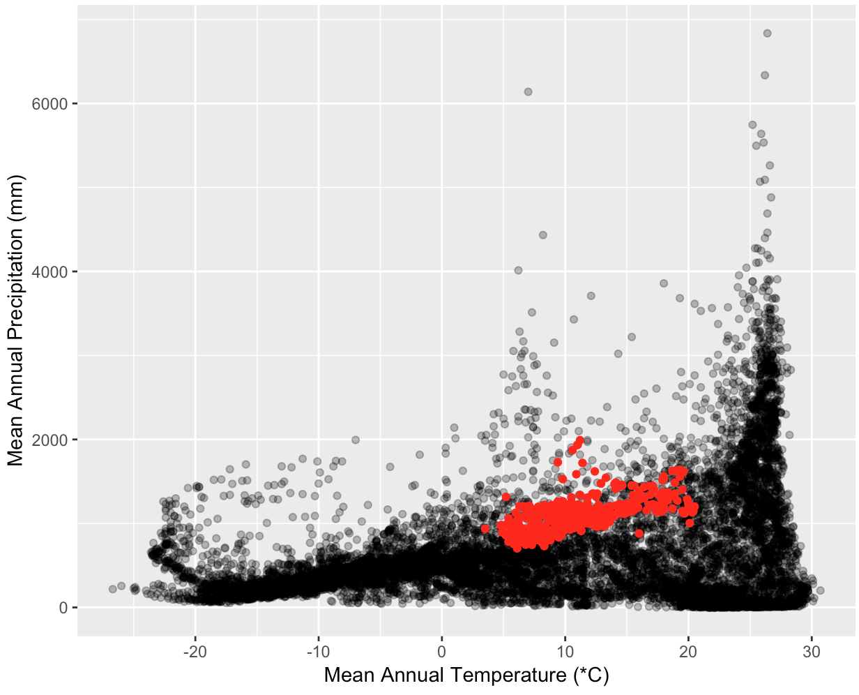
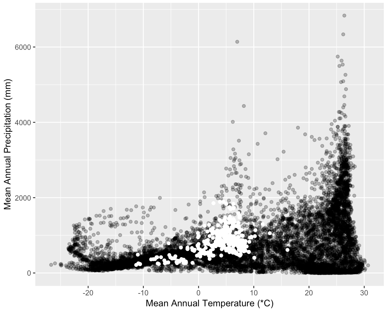
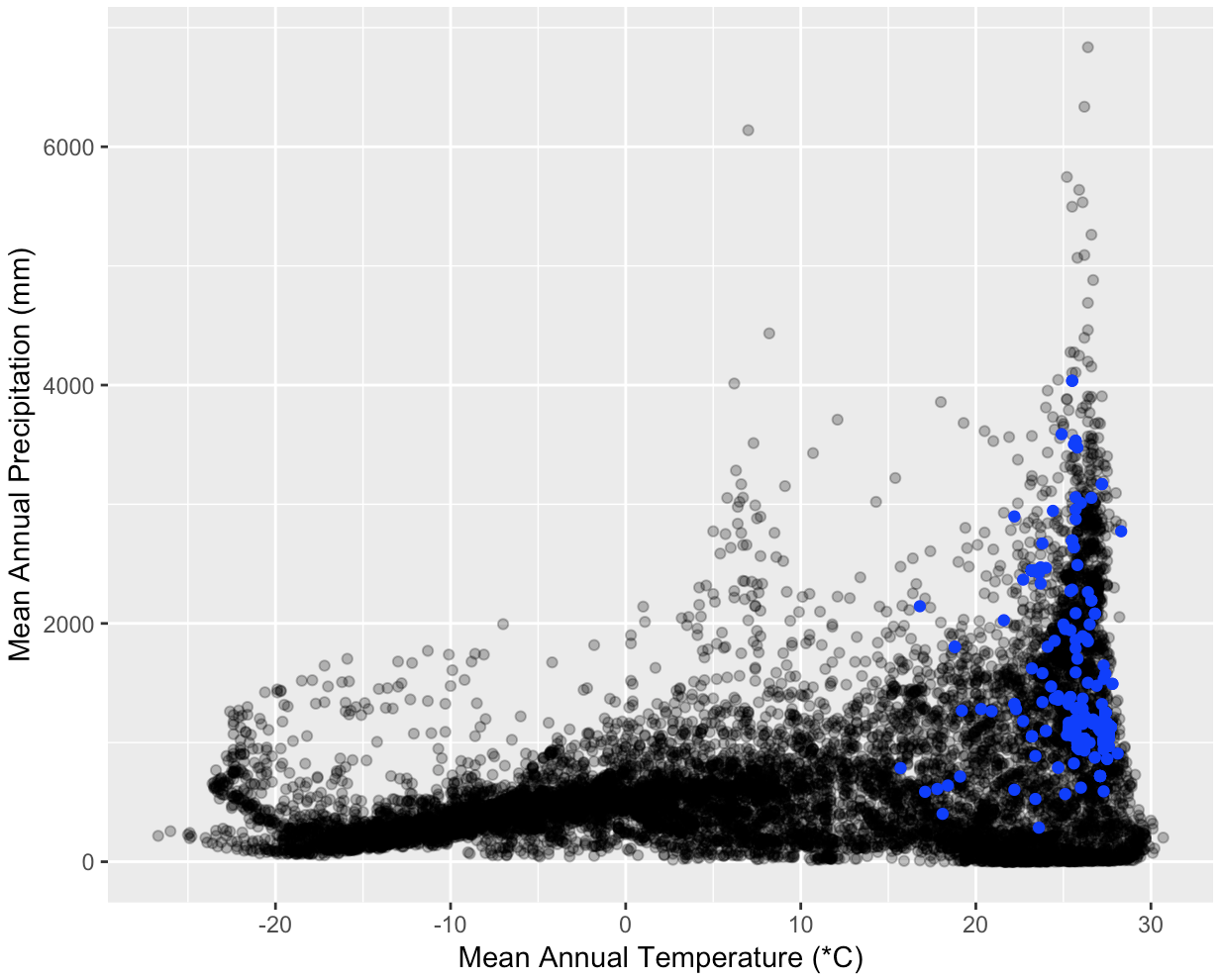
Climate Space (40 pts)
Understanding how environmental factors influence species distributions can be aided by determining which areas of the available climate space a species currently occupies. You are interested in showing how much and what part of the available global temperature and precipitation range is occupied by some common tree species. Create three graphs, one each for Quercus alba, Picea glauca, and Ceiba pentandra. Each graph should show a scatterplot of the mean annual temperature and mean annual precipitation for points around the globe and highlight the values for 1000 locations of the plant species. Start by decomposing this exercise into small manageable pieces.
Here are some tips that will be helpful along the way:
- Climate data data is available from the WorldClim
dataset. Using
climate <- getData('worldclim', var ='bio', res = 10)(from therasterpackage) will download all of the bioclim variables. The two variables you need arebio1(temperature) andbio12(precipitation). If the website is down you can download a copy from the course site by downloading http://www.datacarpentry.org/semester-biology/data/wc10.zip and unzipping it into your home directory (/home/usernameon Mac and Linux,C:\Users\username\Documentson Windows). - There are over 500,000 global data points which can make plotting slow. You
can choose to plot a random subset of 10,000 points (e.g., using
sample_nfrom thedplyrpackage) to limit the time it takes to generate. - Choose good labels and make the points transparent to see their density.
- You might notice that the temperature values seem large. Storing decimal values uses more space than integers, so the WorldClim creators provide temperature values multiplied by 10. For example, 19.5 is stored as 195. Make sure to display the actual temperatures, not the raw values provided. See more information about WorldClim units here.
- Species’ occurrence data is available from GBIF
using the
spoccpackage. An example of how to get the data you need is available in the Species Occurrences Map exercise. - To extract climate values for each occurrence from the climate data you will need a dataframe of occurrences that only only contains longitude and latitude columns.
- If the projections for WorldClim and the species occurrence data aren’t the same you will need a SpatialPointsDataframe.
- There are 19 bioclim variables that are stored together in a “raster stack”.
You can either: 1) run
extracton the full object returned bygetDataand then rundata.frameon the result. This will produce a table with one row for each species location and one column for each bioclim variable; or 2) Get the data for a single bioclim variable using the$, e.g.,climate$bio1, and run extract on this single raster.
Challenge (optional): If you want to challenge yourself trying making a single plot with all three species, either all on the same plot of split over three faceted subplots.
[click here for output] [click here for output] [click here for output]- Climate data data is available from the WorldClim
dataset. Using
Megafaunal Extinction (60 pts)
There were a relatively large number of extinctions of mammalian species roughly 10,000 years ago. To help understand why these extinctions happened scientists are interested in understanding if there were differences in the size of the species that went extinct and those that did not. You are going to reproduce the three main figures from one of the major papers on this topic Lyons et al. 2004.
You will do this using a large dataset of mammalian body sizes that has data on the mass of recently extinct mammals as well as extant mammals (i.e., those that are still alive today). Take a look at the metadata to understand the structure of the data.
- Import the data into R. As with most real world data there are a number of issues with this dataset. Try to spot and clean them up during the import process, but understand that it is common to not discover some data issues until you start analyzing the data. Data cleaning is often an iterative process. Print out the structure of the resulting data frame.
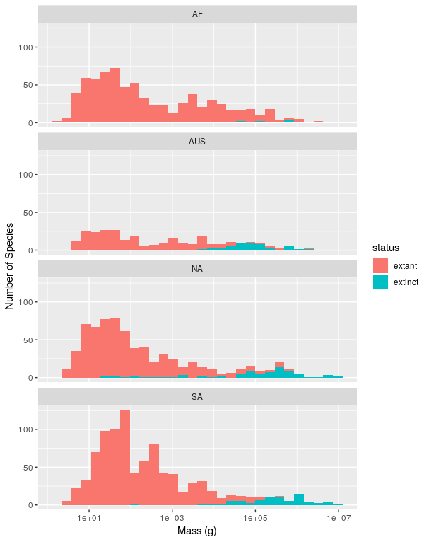
- Create a plot showing histograms of masses for extant mammals and those that
went extinct during the pleistocene (
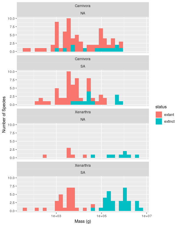
extantandextinctin thestatuscolumn). There should be one sub-plot for each continent and that sub-plot should show the histograms for both groups. Don’t include islands (InsularandOceanicin the `continent column) and only include continents with species that went extinct in the pleistocene. Scale the x-axis logarithmically and stack the sub-plots vertically like in the original paper (but don’t worry about the order of the subplots being the same). Use good axis labels. - The 2nd figure in the original paper looks in more detail at two orders, Xenarthra and Carnivora, which showed extinctions in North and South America. Create a figure similar to the one in Part 2, but that shows 4 sub-plots, one for each order on each of the two continents.
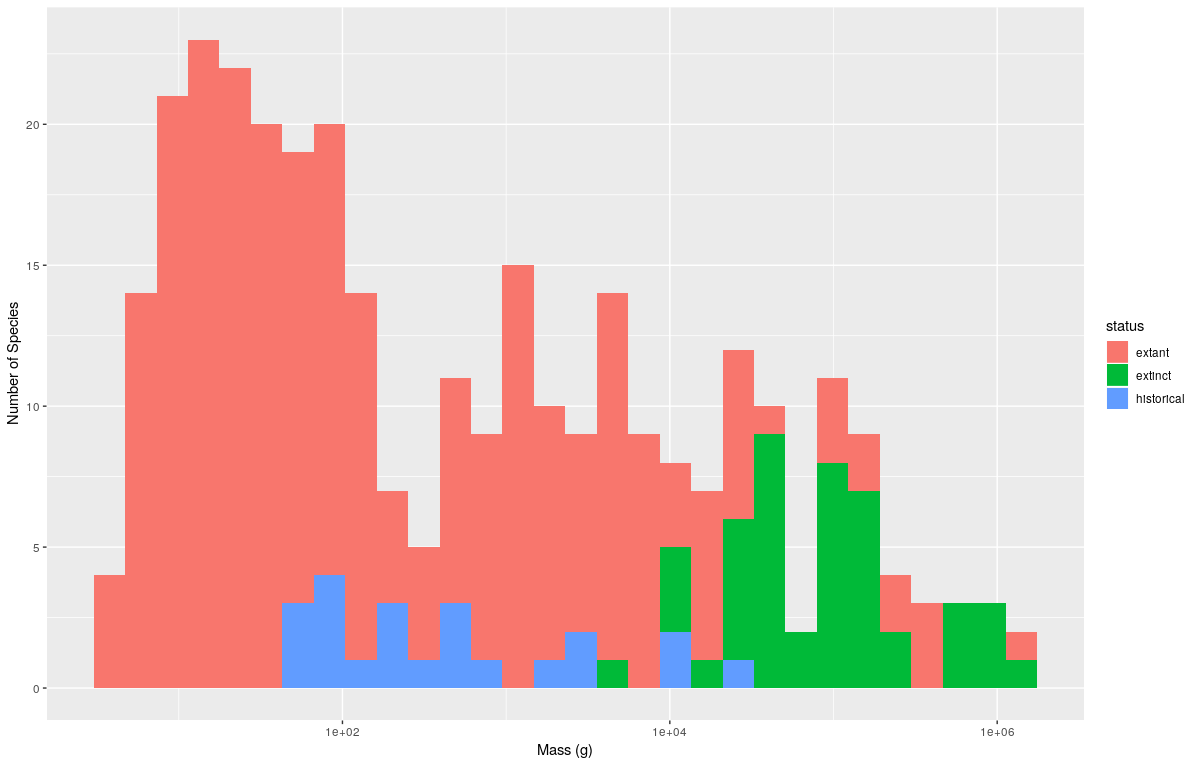
- The 3rd figure in the original paper explores Australia as a case study.
Australia is interesting because there is good data on both Pleistocene
extinctions (
extinctin thestatuscolumn) and more modern extinctions occuring over the last 300 years (historicalin thestatuscolumn). Make a plot similar to the previous plots that compares these three different categoriesextinct,extant, andhistorical). Has the size pattern in exinctions changed for more modern extinctions?